Influence Functions from Scratch

In this post we start from the deceptively simple question:

How does removing a datapoint from the training set influence the model?

There is a fairly elegant series of papers on the topic, which I will summarize.

Analytical Derivation

Suppose we have dataset $X$ with $N$ datapoints $x_i$ and a model with parameters $\Theta$. We then train using empirical risk minimization:

$$L(X, \Theta) = \frac{1}{N} \sum_i L(x_i, \Theta)$$

such that it converges to $\Theta_0 = \argmin_\Theta L(X, \Theta)$.

If we remove a datapoint $x$ from the dataset, we can update the parameters by minimizing:

$$f(\theta) = L(X, \Theta_0 + \theta) - \frac{1}{N} L(x, \Theta_0 + \theta)$$

Taking a second-order Taylor expansion:

$$ \begin{align*} f(\theta) ={}& L(X, \Theta_0) +\underbrace{\nabla_\Theta L(X, \Theta_0)^\mathsf{T}\theta}_{=\;0} + \frac{1}{2}\theta^\mathsf{T}H_{\Theta_0}\theta \\ &- \frac{1}{N}\left[ L(x, \Theta_0) + \nabla_\Theta L(x, \Theta_0)^\mathsf{T}\theta + \frac{1}{2}\underbrace{\theta^\mathsf{T}H_{x,\Theta_0}\theta}_{\mathcal{O}(1/N^2)} \right] \\ &+ \mathcal{O}(\Vert \theta\Vert^3) \end{align*} $$

Then if we assume $\Vert \theta \Vert \in \mathcal{O}(1/N)$ and retain only the terms whose complexity is quadratic in $1/N$:

$$ \begin{align*} f(\theta) \approx {}& L(X, \Theta_0) + \frac{1}{2}\theta^\mathsf{T}H_{\Theta_0}\theta \\ &- \frac{1}{N}\left[ L(x, \Theta_0) + \nabla_\Theta L(x, \Theta_0)^\mathsf{T}\theta \right] \\ \end{align*} $$

Minimizing with first-order optimality conditions gives:

$$\hat{\theta} = \frac{1}{N} H_{\Theta_0}^{-1} \nabla_\Theta L(x, \Theta_0)$$

This basic derivation¹ can be generalized to allow for a loss function with different weighting² of the datapoint:

$$\hat{\theta}(\epsilon) = -\epsilon \cdot H_{\Theta_0}^{-1} \cdot \nabla_\Theta L(x, \Theta_0)$$

This is called an influence function, because it quantifies the first-order effect of a datapoint on the model parameters. The sign of $\epsilon$ modifies whether the datapoint is added or removed from the training set. As a concrete example, say we have a linear model fitted with an OLS loss (for a recap, see this post).

$$L_{\mathrm{OLS}}(X, \beta) = \frac{1}{2} (y - X\beta)^\mathsf{T}(y-X\beta)$$

Thus we obtain the influence of a datapoint $x_i$ on the model parameters $\beta$: $$\hat{\theta}_{\mathrm{OLS}}(\epsilon) = \epsilon \cdot (X^\mathsf{T}X)^{-1} \cdot x_i^\mathsf{T} r_i $$

The inverse-Hessian orients and scales the direction the datapoint pushes the parameters, which for a linear model is the product of the covariate vector with the (scalar) residual. It can be difficult to interpret the influence values directly, so we often convert them into a measurable quantity through additional dot products.

For example, the influence (up to first order) of datapoint $x$ on the model’s loss for test point $z$ is obtained using the chain rule:

$$ \nabla_\epsilon L(z, \Theta_0 + \hat{\theta}(\epsilon)) = -\nabla_\Theta L(z, \Theta_0)^\mathsf{T} \cdot H_{\Theta_0}^{-1} \cdot \nabla_\Theta L(x, \Theta_0)$$

In the linear case, if we set $z=x$ we get a value proportional to the datapoint’s leverage, defined as $P_{ii} = x^\mathsf{T} (X^\mathsf{T}X)^{-1} x$, indicating whether its covariates are far from the bulk of the training data.

In practice, hard-to-classify points can have a large influence on test points because their gradients have high magnitudes. A fix is to normalize $\hat{\theta}$ so only the cosine similarity matters, resulting in a relative influence on the test point.

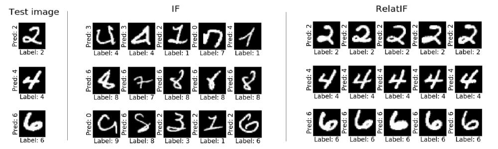
Consider the image above, copied from the RelatIF paper³, comparing the top-5 positively influential images for test points in the MNIST dataset. While the standard influence function recovers handwritten digits with unusual shapes, the relative influence function identifies numbers that look similar to the test image.

Practical Approximations

The influence function $\hat{\theta}$ relies on computing the inverse-Hessian vector product (IHVP). Unfortunately, this is intractable for large models and requires specialized techniques.

We can use the fact that in machine learning, losses are usually probabilistic, e.g. the mean-squared error for regression and the cross-entropy for classification. Under maximum likelihood, we minimize the negative log-likelihood:

$$L(X, \Theta) = -\mathbb{E}_{X|\Theta} \left[ \log p(x | \Theta) \right]$$

so the Hessian is:

$$H = -\nabla_\Theta^2 \mathbb{E}_{X|\Theta} \left[ \log p(x | \Theta) \right]$$

We can make a series of simplifications, first by applying the dominated convergence theorem to swap the order of the expectation and derivatives, then using the fact that the integral of a probability density function is a constant. For brevity, let’s keep $x$ and $\Theta$ implicit in the probability density and gradient operator.

$$ \begin{align*} H &= -\nabla^2 \mathbb{E}_{X|\Theta} \left[ \log p \right] \\ &= -\mathbb{E}_{X|\Theta} \left[ \nabla^2 \log p \right] \\ &= -\mathbb{E}_{X|\Theta} \left[ \nabla \cdot \frac{\nabla p}{p} \right] \\ &= -\mathbb{E}_{X|\Theta} \left[ \frac{(\nabla^2 p)\cdot p - \left( \nabla p \right)\left( \nabla p \right)^\mathsf{T}}{p^2} \right] \\ &= -\underbrace{\int \nabla^2 p \cdot dx}_{=0} + \mathbb{E}_{X|\Theta} \left[\frac{\nabla p}{p} \cdot \frac{\nabla p^\mathsf{T}}{p} \right] \\ &= \mathbb{E}_{X|\Theta} \left[\left( \nabla \log p \right)\left( \nabla \log p \right)^\mathsf{T} \right] \\ &= F \end{align*} $$

We see the Hessian equals the Fisher information matrix⁴. Dropping the $\nabla^2 p$ term is exact in this case, but for non-probabilistic models it would yield the Gauss-Newton approximation of the Hessian⁵.

In practice, we have to work with a finite sample, so we use the empirical Fisher information matrix:

$$F \approx \frac{1}{N} \sum_i \nabla_\Theta \log p(x_i | \Theta) \cdot \nabla_\Theta \log p(x_i | \Theta)^\mathsf{T}$$

This leaves the problem of inverting $F$, which has cubic time complexity in the number of parameters, yet we want to use this method on models with millions of parameters. In deep neural networks, a good option is to group parameters by layer. Denoting gradient vectors as $\mathcal{D}\Theta = \nabla_{\mathrm{vec}(\Theta)} L(x, \Theta)$ where $\mathrm{vec}$ flattens in column-major order, the Fisher for a model with parameters $\Theta = \left[W_1, \ldots, W_B\right]$ forms $B\times B$ blocks:

$$ F = \begin{bmatrix} \mathbb{E}_{X|\Theta}[\mathcal{D}W_1\cdot \mathcal{D}W_1^\mathsf{T}] &\cdots & \mathbb{E}_{X|\Theta}[\mathcal{D}W_1\cdot \mathcal{D}W_B^\mathsf{T}] \\ \vdots & \ddots & \vdots \\ \mathbb{E}_{X|\Theta}[\mathcal{D}W_B\cdot \mathcal{D}W_1^\mathsf{T}] & \cdots & \mathbb{E}_{X|\Theta}[\mathcal{D}W_B\cdot \mathcal{D}W_B^\mathsf{T}] \\ \end{bmatrix} \\ $$

The standard MLP layer is a function $\textrm{MLP}_i(a_{i-1}, W_i) = f(W_i \cdot a_{i-1})$ where $a_{i-1}$ is the activation from the previous layer and $f$ is an element-wise nonlinearity. To compute the Fisher matrix for MLP-style layers:

$$ \begin{align*} \mathcal{D}W_i &= \nabla_{\mathrm{vec}(W_i)} L(x, \Theta) \\ &= \mathrm{vec}\left(\left[\frac{\partial L}{\partial f_i} \odot f^\prime(z_i)\right] \cdot \frac{\partial z_i}{\partial W_i}\right)\\ &= \mathrm{vec}\left(g_i \cdot a_{i-1}^\mathsf{T}\right)\\ &= a_{i-1} \otimes g_i \end{align*} $$

where $g_i$ is the gradient of the loss with respect to the pre-activation embedding $z_i = W_i \cdot a_{i-1}$.

The Kronecker product of matrices with shapes $a\times b$ and $c\times d$ results in a $(a\cdot c) \times (b\cdot d)$-shaped matrix, as the first matrix controls how the second one is stacked. Hence, block $(i,j)$ of the Fisher matrix is:

$$ \begin{align*} F_{i,j} &= \mathbb{E}_{X|\Theta} \left[ \mathcal{D}W_i \cdot \mathcal{D}W_j^\mathsf{T} \right] \\ &= \mathbb{E}_{X|\Theta} \left[ \underbrace{\left(a_{i-1} \otimes g_i\right)}_{(n\cdot m)\times 1} \cdot \underbrace{\left(a_{j-1} \otimes g_j\right)^\mathsf{T}}_{1\times (q\cdot p)} \right] \\ &= \mathbb{E}_{X|\Theta} \left[ \underbrace{(a_{i-1} \cdot a_{j-1}^\mathsf{T})}_{n\times q} \otimes \underbrace{(g_i \cdot g_j^\mathsf{T})}_{m\times p} \right] \end{align*} $$

where $W_i \in \mathbb{R}^{m\times n}$ and $W_j \in \mathbb{R}^{p\times q}$, so $a_{i-1}\in \mathbb{R}^{n\times 1}$, $g_i\in \mathbb{R}^{m\times 1}$, $\mathcal{D}W_i \in \mathbb{R}^{(n\cdot m)\times 1}$, etc.

With the Fisher matrix in block form, we can apply an interesting approximation:

$$ \begin{align*} F_{i,j} &= \mathbb{E}_{X|\Theta} \left[ (a_{i-1} \cdot a_{j-1}^\mathsf{T}) \otimes (g_i \cdot g_j^\mathsf{T}) \right] \\ & \\ &\approx \underbrace{\mathbb{E} \left[a_{i-1} \cdot a_{j-1}^\mathsf{T}\right]}_A \otimes \underbrace{\mathbb{E} \left[g_i \cdot g_j^\mathsf{T}\right]}_G \end{align*} $$

This is K-FAC, the Kronecker-factored approximation of the Fisher matrix, proposed by Martens and Grosse⁶. Recall that the covariance of two random variables is

$$ \mathrm{Cov}(X,Y) = \mathbb{E}[XY] - \mathbb{E}[X]\mathbb{E}[Y]. $$

The Kronecker factorization is therefore exact only if entries of the random matrix $a_{i-1}a_{i-1}^{\mathsf T}$ are uncorrelated with entries of the random matrix $g_i g_i^{\mathsf T}$. Intuitively, if examples with large activation magnitudes also systematically have large pre-activation gradient magnitudes, then the discarded covariance terms may be large and the approximation may perform poorly.

Focusing on a single layer so we can drop subscripts, suppose we eigen-decompose its K-FAC block:

$$ \begin{align*} \text{K-FAC} &= \frac{1}{N} \sum \left[a \cdot a^\mathsf{T}\right] \otimes \frac{1}{N} \sum \left[g \cdot g^\mathsf{T}\right] \\ &= \left(U_A \Lambda_A U_A^\mathsf{T}\right) \otimes \left(U_G \Lambda_G U_G^\mathsf{T}\right) \\ &= \left(U_A \otimes U_G\right) \left(\Lambda_A \otimes \Lambda_G\right) \left(U_A \otimes U_G\right)^\mathsf{T} \\ \end{align*} $$

Refer to $U_A \otimes U_G$ as the Kronecker-Factored Eigenbasis (KFE) with eigenvectors along the columns.

Evidently, K-FAC performs PCA twice, once over inputs and once over gradients with respect to outputs. In the linear regression example we looked at before, this corresponds to eigen-decomposing $\mathbb{E}[X^\mathsf{T}X]$ then multiplying by the variance of the residuals $\mathbb{E}[r^2]$. This variance is a constant under homoscedasticity, so K-FAC reduces to PCA over inputs up to scale. For multivariate errors, the gradient factor captures which output directions are hard to fit, creating a richer representation. However, any Kronecker factorization will be unable to model input-dependent errors.

A further improvement is to project the Fisher matrix onto the KFE and use its diagonal elements instead of the K-FAC eigenvalues. For shorthand, define $\mathrm{KFE}(a, g) = (U_A^\mathsf{T} \cdot a) \otimes (U_G^\mathsf{T} \cdot g)$:

$$ \begin{align*} \Lambda^*_{ii} &= \left[\left(U_A \otimes U_G\right)^\mathsf{T} F \left(U_A \otimes U_G\right)\right]_{ii} \\ &= \frac{1}{N}\sum \left[\left(U_A \otimes U_G\right)^\mathsf{T}(a\otimes g)\right]_i^2 \\ &= \frac{1}{N}\sum \left[\mathrm{KFE}(a, g)\right]_i^2 \end{align*} $$

This method is called EKFAC, the Eigenvalue-corrected Kronecker Factorization⁷. It decreases the Frobenius norm of the residual with respect to the Fisher matrix, but does not guarantee better performance in general.

The Kronecker product has a useful property for inverting matrices:

$$(A \otimes G)^{-1} = A^{-1} \otimes G^{-1}$$

Now if weight matrices have shape $M\times N$, the time complexity of inverting a block in $F$ is reduced from $\mathcal{O}(M^3N^3)$ to $\mathcal{O}(M^3 + N^3)$. This makes a block-diagonal approximation of the inverse Fisher matrix tractable, assuming curvature interactions between layers are relatively small.

Finally, with all these approximations in place, computing the IHVP is computationally feasible. Such techniques have been applied at scale to study generalization in large language models⁸ and are promising for data filtering and active learning⁹.

Dataset Similarity

The influence function gives us a pairwise measure of similarity between two datapoints $s$ and $t$:

$$\mathcal{I}(s,t) = \nabla_\Theta L(s, \Theta_0)^\mathsf{T} \cdot F^{-1} \cdot \nabla_\Theta L(t, \Theta_0)$$

In the kernel methods literature, this is known as the Fisher kernel¹⁰, and its underlying feature space is $\phi(x) = F^{-\frac{1}{2}} \nabla_\Theta L(x, \Theta_0)$.

We can extend this notion of similarity beyond single datapoints to that of datasets. Suppose the training data is sampled from $p(x) = \int p(x, \gamma) d\gamma$, where $\gamma$ is a latent variable controlling the data’s properties. For example, if the support of $x$ is natural images, we could sample a dataset of bird images from $p(x | \gamma = \text{bird})$.

Define random variables $S\sim p(x | \gamma_s)$ and $T\sim p(x | \gamma_t)$ as samples from two independent datasets with different properties. The influence $\mathcal{I}(S,T)$ is also a random variable. Taking its expectation and applying EKFAC, we get:

$$ \begin{align*} \mathbb{E}[\mathcal{I}(S,T)] &= \mathbb{E} \left[\phi(S) \right]^\mathsf{T} \cdot \mathbb{E} \left[\phi(T)\right] \\ &= \mathbb{E} \left[\nabla_\Theta L(S, \Theta_0) \right]^\mathsf{T} \cdot F^{-1} \cdot \mathbb{E} \left[\nabla_\Theta L(T, \Theta_0)\right] \\ &\approx \mathbb{E}\left[\mathrm{KFE}(a_S, g_S)\right]^\mathsf{T} \cdot (\Lambda^*)^{-1} \cdot \mathbb{E}\left[\mathrm{KFE}(a_T, g_T)\right] \\ \end{align*} $$

In practice, comparing datasets this way requires a shared reference model whose Fisher geometry is meaningful across all of them. This can be achieved by training a large model on a multi-task objective, either explicitly or implicitly through generative tasks like text completion.

Task2Vec¹¹ is a concrete instance. The authors take an ImageNet-pretrained feature extractor (called a probe) as the shared reference and train a task-specific head on each of several species-classification datasets. Each dataset is then embedded by a coarse-grained diagonal approximation of the Fisher matrix in the probe’s parameter basis. The resulting fixed-size vectors capture which parameters have highest influence on the loss for each dataset. Applying cosine similarity over pairs of these embeddings turns out to align with taxonomic distance between the species present in the datasets. This similarity measure is more heuristic than the Fisher kernel, but it works well enough in their setting.

The same machinery shows up in mechanistic interpretability. A paper from Goodfire¹² uses K-FAC to detect memorization in generative Transformers, e.g. when LLMs reproduce passages from famous novels. Recall that $\mathcal{I}(s,t)$ re-weights directions by the inverse Fisher, so low-eigenvalue directions dominate. In very large models, those directions can encode rote memorization and other brittle behaviors, making the Fisher kernel sensitive to surface details. In the layer-22 MLP of OLMo 7B, their experiments show that the bottom 50% of KFE directions activate 23.1% more strongly on memorized data than clean data, while the top 10% activate 21% less.

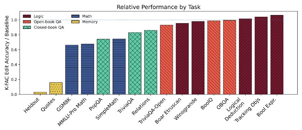
As evident in the plot copied from the paper, editing out components along the bottom 50% suppresses exact recitation of quotes and held-out passages, while preserving boolean logic and open-book QA. The drop in accuracy on GSM8K indicates that the model’s arithmetic abilities are damaged by the edit, suggesting that addition and subtraction are not very robust behaviors.

Altogether, influence functions and the Fisher kernel turn the model’s own loss geometry into a way of comparing datapoints, datasets, and even learned behaviors. I expect there are more useful applications still to be found.